Learning Objectives
By the end of this chapter you will be able to:
- Describe the Demand/Potential/Allocation loop that LuccME established and DisSLUCC keeps
- Choose between continuous and discrete allocation for a given research question
- Build and run a continuous LUCC model in a script, and know the executor and TOML route to the same components
- Say what the comparison with the LuccME test labs shows about DisSLUCC — and what it does not
# Standard imports — add chapter-specific imports below
import numpy as np
import pandas as pd
import matplotlib.pyplot as plt
Every model since Chapter 23 has been a paradigm demonstration — Predator-Prey, Game of Life, a handful of agents. This chapter is the first full domain application: land use and cover change (LUCC), the process that motivated LuccME at INPE/CCST, and the process DisSModel's own migration story (Chapter 34) keeps returning to as its central example.
What DisSLUCC Is
DisSLUCC implements LuccME's components — demand, potential, allocation — in Python, on the raster substrate of DisSModel. It is one package, disslucc, in which the continuous and discrete components live side by side, as they do in LuccME itself. (Earlier drafts of this book used two packages, disslucc-continuous and disslucc-discrete; they were merged into this one.) It is meant to be run next to TerraME and LuccME, which remain the reference, not to replace them.
| Role | Components |
|---|---|
| Demand — how much? | DemandInline, DemandPreComputedValues (a table), DemandComputeTwoDates, DemandComputeThreeDates (from land-use layers) |
| Potential — where? | PotentialLinearRegression (continuous), PotentialSpatialLagRegression (continuous, with a spatial-lag term), PotentialDLogisticRegression (discrete) |
| Allocation — how is the change placed? | AllocationClueLike (continuous, CLUE-like), AllocationClueLikeSaturation (continuous, with saturation), AllocationDClueSLike (discrete, CLUE-S-like) |
Each component is an ordinary DisSModel Model, registered in the same Environment in the order it is built — the lifecycle of Chapter 22, nothing more. There are two entry points to the same components: a script (build the models in Python and call env.run() — the fastest way to experiment) and an executor (disslucc.executors, which wraps the same components in a ModelExecutor with an ExperimentRecord, reads its configuration from a TOML file, and has a command line). Both give the same result; the executor adds the provenance record of Chapter 29.
Theory: Demand, Potential, Allocation
Every LUCC model in this chapter, continuous or discrete, runs the same three-part loop each time step — the structure LuccME took from the CLUE family of models:
- Demand ("how much?") — the area of each land use in this step. It can come from a historical trend, a constructed scenario, an economic model, or simply a precomputed table read from a CSV.
- Potential ("where?") — a suitability map built from driving-factor layers: distance to roads, distance to ports, protected-area status, soil fertility. This is a regression problem — predicting suitability from spatial covariates — with those covariates prepared upstream by DisSCube (Chapter 28).
- Allocation — spatially distributing the demanded area according to the potential map, by iteration until the allocated area meets the demand within a tolerance (
max_difference), or by competition between classes.
Is a land-change model a cellular automaton? By Chapter 24's own six-element definition — grid, neighborhood, finite states, transition rules, initial state, discrete time — yes, formally. The difference from DisSModel CA's models is one of emphasis and disciplinary origin (land-use science, not physics), and one of mechanism: allocation is driven by a demand for the whole region, not by each cell's neighbors alone.
Continuous Allocation
PotentialLinearRegression + AllocationClueLike answer "how much does this cell's land use change" — the right choice whenever a cell can legitimately hold more than one land use at once (a partially deforested cell, a partially urbanized one). Each cell holds a fraction of each class. Potential is one linear regression per land-use type, each with its own intercept and driving-factor coefficients (RegressionSpec); allocation distributes the demand across cells according to that potential, subject to per-class bounds (AllocationSpec).
The example below is the package's own synthetic scenario, run in this notebook: a 30 × 30 grid, mostly forest, with a horizontal road through the middle, a smooth terrain (slope), and one urban seed cell on the road. Two drivers, three classes:
from dissmodel.geo import RasterBackend

LAND_USE_TYPES = ["forest", "agriculture", "urban"]
H = W = 30
rng = np.random.default_rng(42)

road_row = H // 2
dist_road = np.repeat(np.abs(np.arange(H, dtype=np.float32)[:, None] - road_row), W, axis=1)
dist_road /= dist_road.max()                                    # 0 on the road, 1 at the edges

yy, xx = np.mgrid[0:H, 0:W]
slope = (np.sin(xx / 4.0) * 0.5 + np.cos(yy / 5.0) * 0.5 + rng.normal(0, 0.05, (H, W))).astype(np.float32)
slope = (slope - slope.min()) / (slope.max() - slope.min())     # normalised to [0, 1]

backend = RasterBackend(shape=(H, W))
backend.set("dist_road", dist_road.astype(np.float32))
backend.set("slope", slope)
urban = np.zeros((H, W), dtype=np.float32); urban[road_row, W // 2] = 1.0
backend.set("urban", urban)
backend.set("agriculture", np.zeros((H, W), dtype=np.float32))
backend.set("forest", 1.0 - urban)

# Demand: total area per class and step (order of LAND_USE_TYPES); urban and agriculture grow
N_STEPS = 8
demand_matrix = [[float(H * W - (1 + 3 * s) - s), float(s), float(1 + 3 * s)] for s in range(N_STEPS)]
pd.DataFrame(demand_matrix, columns=LAND_USE_TYPES).rename_axis("step").T
| step | 0 | 1 | 2 | 3 | 4 | 5 | 6 | 7 |
|---|---|---|---|---|---|---|---|---|
| forest | 899.0 | 895.0 | 891.0 | 887.0 | 883.0 | 879.0 | 875.0 | 871.0 |
| agriculture | 0.0 | 1.0 | 2.0 | 3.0 | 4.0 | 5.0 | 6.0 | 7.0 |
| urban | 1.0 | 4.0 | 7.0 | 10.0 | 13.0 | 16.0 | 19.0 | 22.0 |
The model is three components in one Environment, built in the order they run each step — demand, then potential, then allocation:
import contextlib, io
from dissmodel.core import Environment
from disslucc import DemandInline, PotentialLinearRegression, AllocationClueLike
from disslucc.schemas import RegressionSpec, AllocationSpec

env = Environment(end_time=N_STEPS - 1)

demand = DemandInline(values=demand_matrix, land_use_types=LAND_USE_TYPES)

potential = PotentialLinearRegression(
    backend=backend, demand=demand, land_use_types=LAND_USE_TYPES,
    potential_data=[[                                                        # one region
        RegressionSpec(const=-0.2, betas={"slope": 0.4}),                    # forest
        RegressionSpec(const=0.4, betas={"dist_road": -0.1, "slope": -0.5}), # agriculture
        RegressionSpec(const=0.3, betas={"dist_road": -0.6, "slope": -0.3}), # urban
    ]],
)

allocation = AllocationClueLike(
    backend=backend, demand=demand, potential=potential, land_use_types=LAND_USE_TYPES,
    static={"forest": 0, "agriculture": -1, "urban": -1},   # forest is free; the others follow demand
    complementar_lu="forest",                                # forest takes whatever the others leave
    cell_area=1.0, max_difference=5.0,                       # stop when within 5 cells of the demand
    allocation_data=[AllocationSpec(static=0), AllocationSpec(static=-1), AllocationSpec(static=-1)],
)

with contextlib.redirect_stdout(io.StringIO()):              # the components log every iteration
    env.run()

for i, lu in enumerate(LAND_USE_TYPES):
    print(f"{lu:>12}: demand {demand_matrix[-1][i]:7.1f}   allocated {float(backend.get(lu).sum()):7.1f}")
      forest: demand   871.0   allocated   866.3
 agriculture: demand     7.0   allocated    11.3
       urban: demand    22.0   allocated    22.3
fig, axes = plt.subplots(1, 3, figsize=(11, 3.6))
for ax, lu in zip(axes, LAND_USE_TYPES):
    im = ax.imshow(backend.get(lu), cmap="viridis", vmin=0, vmax=1)
    ax.set_title(lu); ax.set_axis_off()
fig.colorbar(im, ax=axes, shrink=0.8, label="share of the cell")
fig.suptitle(f"Land use after {N_STEPS} steps (synthetic scenario)")
plt.show()

The allocated areas meet the demand of the last step within the tolerance of 5 cells (forest ends 4.7 cells below its demand and agriculture 4.3 above — a small gap in absolute terms, but more than half of agriculture's own demand of 7, a reminder that a tolerance set for the whole grid says little about a small class). Urban land grows out from the seed along the road, where dist_road is small and its coefficient is most negative; agriculture spreads thinly around the same corridor, and forest gives up what the other two take, as complementar_lu says. Nothing here is calibrated: the coefficients were chosen to make the mechanism visible.
Two continuous variants matter for real models. PotentialSpatialLagRegression adds to the regression a term ro times the mean of the class in the neighboring cells, so that change is drawn towards where the class already is; AllocationClueLikeSaturation limits how fast a cell can change once it passes a threshold. LuccME-BR, the national model behind Chapter 31, uses both.
Discrete Allocation
PotentialDLogisticRegression + AllocationDClueSLike answer a different question: "which single land use dominates this cell" — a CLUE-S-style allocation, right whenever the data are themselves categorical (a classified land-cover map, not a fractional-cover raster). Potential comes from a logistic regression predicting which class a cell most likely belongs to (LogisticRegressionSpec, which adds an elasticity term — how hard a class is to remove from a cell); allocation runs a competition between classes, governed by a transition matrix ([region][from][to]: which changes are allowed at all).
The executor route reads the same configuration from a TOML file — the format Chapter 33's platform registers — and runs it from the command line. The package's example for the Moju region:
[model]
executor_module   = "disslucc.executors"
name              = "lucc_discrete"
land_use_types    = ["f", "d", "o"]
cell_area         = 1.0
transition_matrix = [[[1, 1, 0], [0, 1, 0], [0, 0, 1]]]   # deforestation is irreversible

[model.parameters]
n_steps          = 6
max_difference   = 100.0
factor_iteration = 0.0001

[[model.potential_data]]
lu         = "f"
const      = -2.34187976925989
elasticity = 0.0
  [model.potential_data.betas]
  dist_br = 3.10319957497883
git clone https://github.com/DisSModel/disslucc.git && cd disslucc
pip install -e ".[examples]"
python -m disslucc.executors.discrete run \
  --toml examples/dissmodel-configs/lucc_discrete.toml \
  --input data/input/cs_moju.zip \
  --param demand_csv=data/input/demand_moju.csv \
  --output outputs/result.tif
--output writes a GeoTIFF with one band per land-use class, georeferenced from the input, and the run leaves an ExperimentRecord with the checksums of the input and the output. One caveat comes with this route: the executor rasterizes the input layer at the resolution given in the TOML, so its grid is close to, but not cell for cell the same as, the original cellular space (5,842 of the 5,914 cells of Moju). That is why the comparison with LuccME below builds each model by hand on the lab's own cells, not through the executor.
Choosing Between Continuous and Discrete
Both styles implement the same Demand/Potential/Allocation loop with different algorithms at each step — the decision between them is about your data, not architecture:
| Continuous | Discrete | |
|---|---|---|
| A cell holds | a fraction of each class | one class |
| Potential | linear regression (optionally with a spatial lag) | logistic regression |
| Allocation | CLUE-like, per-class bounds, optional saturation | CLUE-S competition, transition matrix |
| Natural comparison with a reference | tolerance on fractions | agreement of classes, cell by cell |
The fastest way to decide: look at your calibration and validation data first. If they are a class label per cell, discrete allocation is what can be checked against them directly. If they are an area or a share per cell, continuous allocation represents them without a lossy discretization forced on them first.
Checked Against LuccME
Writing LuccME's components again in another language is only useful if they compute what the originals compute. The package does not check that itself: a separate repository, disslucc-benchmark, runs DisSLUCC on the test labs that ship with LuccME 3.1 and compares the result, cell by cell and year by year, with the outputs TerraME 2.0.1 produced for the same labs, archived in luccme-goldens. Chapter 30 explains how those reference outputs were produced and checked; here are the results.
LuccME 3.1 ships 21 test labs. DisSLUCC implements every component of ten of them — lab01 to lab07 (continuous, Acre, 6,574 cells) and lab15 to lab17 (discrete, Moju, 5,914 cells) — and those ten match the TerraME outputs with the same number of allocation iterations in every year and a largest cell difference between 5×10⁻¹³ and 3×10⁻⁶, the larger values coming from single-precision arithmetic. The other eleven labs use components DisSLUCC does not have yet: seven lack one component each, four need several.
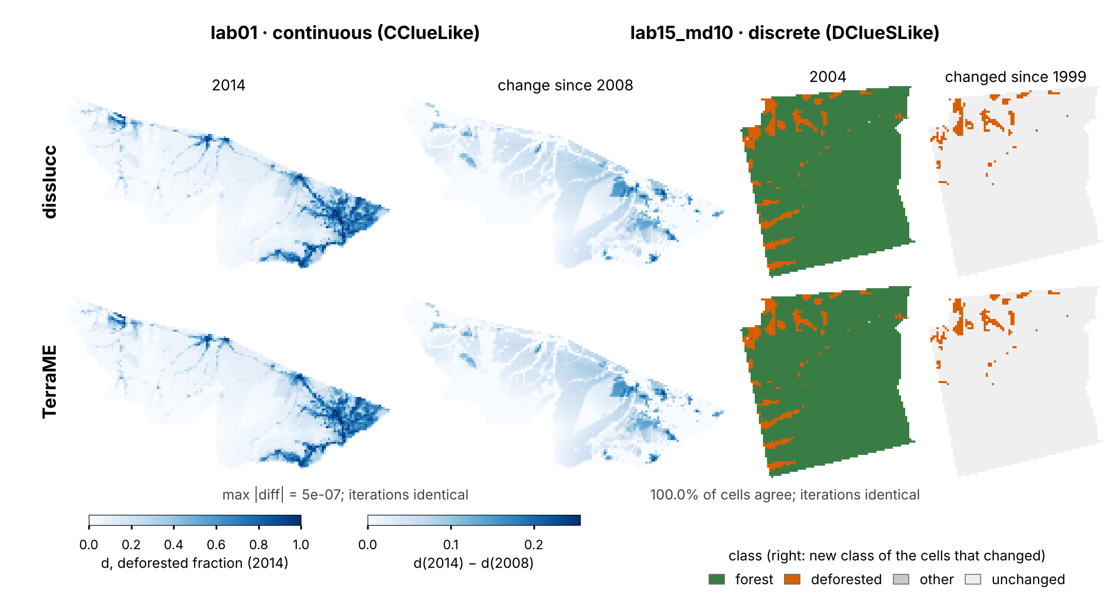
A continuous and a discrete LuccME lab, DisSLUCC 0.5.0 (top row) against the TerraME 2.0.1 output (bottom row), on the same cells and with the same color limits. Left, lab01: the deforested fraction in 2014 and its change since 2008. Right, lab15_md10: the class of each cell in 2004 and the 237 cells that changed class since 1999. The two rows are not expected to be distinguishable by eye. From disslucc-benchmark, docs/fig_models.png.
Three details of this comparison are worth more than the headline.
The labs barely exercise the convergence loop. In the ten labs as shipped, the allocation is accepted at the first pass every year, so "same number of iterations" says little. The benchmark adds two variants with a smaller maxDifference, in which the loop runs 8 to 67 times per year: lab01_md1643 (continuous) and lab15_md10 (discrete). DisSLUCC reproduces TerraME's iteration count in every year of both. The second answers an old caveat of this chapter: with its original maxDifference of 300, lab15 is nearly non-discriminative — no cell changes class, and a static ranking by the difference of two probabilities already reproduces it — so its match only showed that the coefficients were transcribed correctly. In lab15_md10, 237 cells change class, the competition between classes matters, and every cell still agrees.
One difference is deliberate. LuccME's continuous allocation contains a correction of the change in each cell that never runs: the condition that guards it reads a field named regionregionAloc instead of regionAloc, so it is always false. DisSLUCC runs the correction by default, as the algorithm intends, and has a switch, AllocationClueLike(cell_correction=False), that reproduces LuccME exactly. With the correction on, lab01 with maxDifference 1643 differs from TerraME by a mean of 0.0036 in the forest and deforested fractions in 2014 (largest 0.027), and the iteration counts change. An earlier draft of this chapter reported that 0.0036 as the agreement of DisSLUCC with LuccME and blamed it on the convergence tolerance; it is in fact entirely this correction, and with the switch off the difference disappears.
Parity is not validation of a model. All of this shows that DisSLUCC's components compute what LuccME's compute, on the labs, to the precision measured. It does not show that the labs are good models of Acre or Moju, nor that LuccME itself is right. Those are the questions of the next section.
Calibration, Validation, and Goodness-of-Fit
The comparison above is engineering validation — confirming that a Python implementation matches a reference run. That is a different question from scientific validation: fitting a model to real-world observed data by splitting a timeline into a calibration period (used to fit the parameters) and a held-out validation period, checked only after fitting.
A cell-by-cell comparison between a simulated map and an observed one is often too strict a bar even for scientific validation — two reasonable model runs can disagree pixel for pixel while still being "equally good" at the pattern level. A multiscale comparison — checking agreement in successively larger windows (3×3, then 5×5, then 9×9, and so on) — is the standard alternative: two maps might show weak agreement at the finest resolution but strong agreement at a coarser one, which is real, usable information a strict pixel match would have discarded. For categorical maps, the Pontius & Millones decomposition into quantity and allocation disagreement — available in disslucc.validation.pontius_millones — says how two maps disagree, which a single accuracy number hides.
Exercises
- Match the component to the question. For each research question, name which allocation style fits and why: (a) "how does the percentage of forest cover in each cell change over the next 20 years," (b) "which cells convert from forest to pasture by 2030."
- Why two different regressions?
PotentialLinearRegressionandPotentialDLogisticRegressionboth take driving-factor coefficients (betas) per land-use type. From the class names alone, explain why one needs a linear regression and the other a logistic one — what is each one actually trying to predict? - Move the road. In the synthetic scenario, change the
urbancoefficient ofdist_roadfrom −0.6 to +0.6 and run it again. Where does urban land go now, and does the allocation still meet the demand? - Tolerance and iterations. Run the scenario with
max_difference=0.5instead of 5.0. Does the allocated area get closer to the demand? Why does a smaller tolerance make a comparison of iteration counts with a reference more informative? - Read a deliberate difference. In your own words, explain why the benchmark keeps
lab01/cell_correctionas a scenario that is expected to differ from TerraME, instead of removing it.
# Your code here
Summary
Key concepts introduced
- DisSLUCC: one raster package with LuccME's demand, potential and allocation components, continuous and discrete, meant to run next to LuccME rather than replace it
- The Demand/Potential/Allocation loop, and the components that fill each role, including the spatial-lag potential and saturation allocation used at national scale
- A continuous model built and run in a script; the executor and TOML route to the same components, with its command line and its provenance record
- Choosing continuous or discrete allocation by the type of your data
- The comparison with ten of the 21 LuccME labs: identical iteration counts, differences at single-precision level, two variants that make the convergence loop and the class competition matter, and one deliberate difference (the cell correction LuccME never runs)
- Engineering validation against a reference versus scientific validation against observations
Chapter 27 stays in domain-application territory but moves from land far inland to the coastline itself — a coupled flood and mangrove-migration model, run on both substrates and validated two different ways at once.
Further Reading
- Costa, S. S. (2026). DisSLUCC (Version 0.5.0) [Computer software]. Zenodo. https://doi.org/10.5281/zenodo.23219338
- Costa, S. S. (2026). DisSLUCC benchmark (Version 0.2.2) [Computer software]. Zenodo. https://doi.org/10.5281/zenodo.23224097 — the comparison with the LuccME labs
- Veldkamp, A., & Fresco, L. O. (1996). CLUE: a conceptual model to study the conversion of land use and its effects. Ecological Modelling, 85(2–3), 253–270
- Verburg, P. H. et al. (2002). Modeling the spatial dynamics of regional land use: the CLUE-S model. Environmental Management, 30(3), 391–405
- Costanza, R. (1989). Model goodness of fit: a multiple resolution procedure. Ecological Modelling, 47(3–4), 199–215 — the multiscale comparison
- Pontius Jr., R. G. & Millones, M. (2011). Death to Kappa: birth of quantity disagreement and allocation disagreement for accuracy assessment. International Journal of Remote Sensing, 32(15), 4407–4429
- LuccME documentation (INPE): http://www.dpi.inpe.br/luccme/